Chapter 2 Probability: When an Outcome is Unknown
Status: needs some elaborating and some good examples. See Section 1.1.
Imagine what life would be like if nothing was certain. If you let go of a ball, sometimes it falls, stays put, or adopts some other motion. If you wrap yourself in a blanket, sometimes it warms you up, and sometimes it cools you down. Or, taking pain medicine sometimes eases your pain, and sometimes makes it worse. Indeed, we rely on known cause-and-effect relationships in order to operate day to day. And whatever cause-and-effect relationships we don’t know, we can learn them to allow us to expand our ability to operate in this world of ours. Don’t know how to ski? Just learn the motions that will result in you descending a snowy mountain with control and a lot of fun.
But there are many things that are in fact uncertain. Maybe your income relies on how many clients you get, so that you don’t even know your income next month. Maybe you don’t know whether breast feeding your baby will result in less colic than bottle feeding, because you’ve seen your friends’ colicky babies in both cases. Does uncertainty mean we should resort to claiming ignorance? That you have no idea what your income will be in a month? That it’s impossible to know whether the way your baby is fed impacts colic? These might sound like realistic claims holding a rudimentary cause-and-effect mindset, but the reality is that we often can in fact garner information from uncertain outcomes if we adopt a probabilistic mindset.
When the result of an outcome is known, it is referred to as deterministic, whereas an unknown outcome is referred to as stochastic. To understand a stochastic outcome and what influences it, it’s key to understand probability distributions, which are the topic of this chapter.
2.1 Probability Distributions
Before abstracting probability distributions to real examples, it’s perhaps best to explore probability distributions using simple examples where probabilities are known.
A probability distribution is a complete indication of how much probability is associated with certain outcomes.
If we roll a 6-sided die, since each of the six outcomes (the numbers 1 through 6) are equally likely, each outcome has a probability of 1/6. The distribution of the dice roll is the specification of probabilities for each outcome:
| Outcome | Probability |
|---|---|
| 1 | 1/6 |
| 2 | 1/6 |
I like to play Mario Kart 8, a racing game with some “combat” involved using items. In the game, you are given an item at random whenever you get an “item box”.
Suppose you’re playing the game, and so far have gotten the following items in total:
| Item | Name | Count |
|---|---|---|
 |
Banana | 7 |
 |
Bob-omb | 3 |
 |
Coin | 37 |
 |
Horn | 1 |
 |
Shell | 2 |
| Total: | 50 |
Attribution: images from pngkey.
2.1.1 Probability
- What’s the probability that your next item is a coin?
- How would you find the actual probability?
- From this, how might you define probability?
In general, the probability of an event \(A\) occurring is denoted \(P(A)\) and is defined as \[\frac{\text{Number of times event } A \text{ is observed}}{\text{Total number of events observed}}\] as the number of events goes to infinity.
2.1.2 Probability Distributions
So far, we’ve been discussing probabilities of single events. But it’s often useful to characterize the full “spectrum” of uncertainty associated with an outcome. The set of all outcomes and their corresponding probabilities is called a probability distribution (or, often, just distribution).
The outcome itself, which is uncertain, is called a random variable. (Note: technically, this definition only holds if the outcome is numeric, not categorical like our Mario Kart example, but we won’t concern ourselves with such details)
When the outcomes are discrete, the distributions are called probability mass functions (or pmf’s for short).
2.1.3 Examples of Probability Distributions
Mario Kart Example: The distribution of items is given by the above table.
Ship example: Suppose a ship that arrives at the port of Vancouver will stay at port according to the following distribution:
| Length of stay (days) | Probability |
|---|---|
| 1 | 0.25 |
| 2 | 0.50 |
| 3 | 0.15 |
| 4 | 0.10 |
The fact that the outcome is numeric means that there are more ways we can talk about things, as we will see.
2.2 Continuous random variables (10 min)
What is the current water level of the Bow River at Banff, Alberta? How tall is a tree? What about the current atmospheric temperature in Vancouver, BC? These are examples of continuous random variables, because there are an uncountably infinite amount of outcomes. Discrete random variables, on the other hand, are countable, even if there are infinitely many outcomes, because each outcome can be accounted for one-at-a-time by some pattern.
Example: The positive integers are discrete/countable: just start with 1 and keep adding 1 to get 1, 2, 3, etc., and that covers all possible outcomes. Positive real numbers are not countable because there’s no way to cover all possibilities by considering one outcome at a time.
It turns out that it’s trickier to interpret probabilities for continuous random variables, but it also turns out that they’re in general easier to work with.
Not all random variables with infinitely many outcomes are continuous. Take, for example, a Poisson random variable, that can take values \(0, 1, 2, \ldots\) with no upper limit. The difference here is that a smaller range of values does have a finite amount of variables. By the way, this type of infinity is called “countably infinite”, and a continuous random variable has “uncountably infinite” amount of outcomes.
2.2.0.1 Advanced and Optional: Is anything actually continuous?
In practice, we can never measure anything on a continuous scale, since any measuring instrument must always round to some precision. For example, your kitchen scale might only measure things to the nearest gram. But, these variables are well approximated by a continuous variable. As a rule of thumb, if the difference between neighbouring values isn’t a big deal, consider the variable continuous.
Example:
You’d like to get a handle on your monthly finances, so you record your total monthly expenses each month. You end up with 20 months worth of data:
##  [1] "$1903.68" "$3269.61" "$6594.05" "$1693.94" "$2863.71" "$3185.01"
##  [7] "$4247.04" "$2644.27" "$8040.42" "$2781.11" "$3673.23" "$4870.13"
## [13] "$2449.53" "$1772.53" "$7267.11" "$938.67"  "$4625.33" "$3034.81"
## [19] "$4946.4"  "$3700.16"
Since a difference of $0.01 isn’t a big deal, we may as well treat this as a continuous random variable.
Example:
Back in the day when Canada had pennies, you liked to play “penny bingo”, and wrote down your winnings after each day of playing the game with your friends. Here are your net winnings:
## [1] 0.01 -0.01 0.02 0.01 0.04 0.02 -0.03 -0.01 0.05 0.04Since a difference of $0.01 is a big deal, best to treat this as discrete.
2.3 Density Functions (20 min)
In the discrete case, we were able to specify a distribution by indicating a probability for each outcome. Even when there’s an infinite amount of outcomes, such as in the case of a Poisson distribution, we can still place a non-zero probability on each outcome and have the probabilities sum to 1 (thanks to convergent series). But an uncountable amount of outcomes cannot be all accounted for by a sum (i.e., the type of sum we denote by \(\sum\)), and this means that continuous outcomes must have probability 0.
Example: The probability that the temperature in Vancouver tomorrow will be 18 degrees celcius is 0. In fact, any temperature has a probability of 0 of occurring.
While individual outcomes have zero probability, ranges can have non-zero probability. We can use this idea to figure out how “dense” the probability is at some areas of the outcome space. For example, if a randomly selected tree has a 0.05 probability of being within 0.1m of 5.0m, then as a rate, that’s about 0.05/(0.1m) = 0.5 “probability per meter” here. Taking the limit as the range width \(\rightarrow 0\), we obtain what’s called the density at 5m.
The density as a function over the outcome space is called the probability density function (pdf), usually abbreviated to just the density, and denoted \(f\). Sometimes we specify the random variable in the subscript, just to be clear about what random variable this density represents – for example, \(f_X\) is the density of random variable \(X\).
You’ll see that the density is like a “continuous cousin” of the probability mass function (pmf) in the case of discrete random variables. We’ll also see in a future lecture that there are some random variables for which neither a density nor a pmf exist.
We can use the density to calculate probabilies of a range by integrating the density over that range: \[P(a < X < b) = \int_a^b f(x) \text{d}x.\] This means that, integrating over the entire range of possibilities should give us 1: \[\int_{-\infty}^\infty f(x) \text{d}x = 1\] This integral corresponds to the entire area under the density function.
2.3.1 Example: “Low Purity Octane”
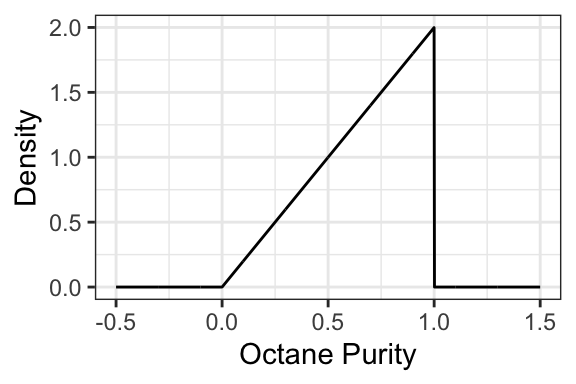
You just ran out of gas, but luckily, right in front of a gas station! Or maybe not so lucky, since the gas station is called “Low Purity Octane”. They tell you that the octane purity of their gasoline is random, and has the following density:

- What’s the probability of getting 25% purity? That is, \(P(\text{Purity} = 0.25)\)?
- The density evaluates to be >1 in some places. Does this mean that this is not a valid density? Why is the density in fact valid?
- Is it possible for the density to be negative? Why or why not?
- What’s the probability of getting gas that’s \(<50\%\) pure? That is, \(P(\text{Purity} < 0.5)\)?
- What’s the probability of getting gas that’s \(\leq 50\%\) pure? That is, \(P(\text{Purity} \leq 0.5)\)?
- What’s the support of this random variable? That is, the set of all outcomes that have non-zero density?
- You decide to spend the day at Low Purity Octane, measuring the octane purity for each customer. You end up getting 100 observations, placing each measurement along the x-axis. Which of the following plots would be more likely, and why?

2.3.2 Example: Monthly Expenses
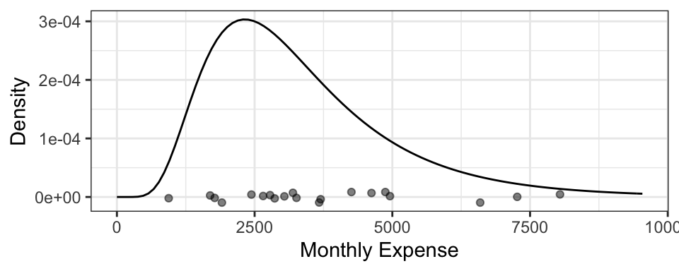
It turns out your monthly expenses have the following density, with your 20 observations plotted below it:

2.4 Summary and take-aways
- These distributions might not seem practical, but they certainly are. Even in cases where we are considering many other pieces of information aside from the response, we are still dealing with univariate distributions – we’ll see later that the only difference is that they are no longer marginal distributions (they are conditional).
- It’s important to consider whether you are interested in the result of a single observation, or whether you are more interested in outcomes observed in the long run. While Statistics uses repeated observations in the long run to identify patterns and distributions, how you use those distributions will depend on your interest.